Supervised machine learning

26/05/2025

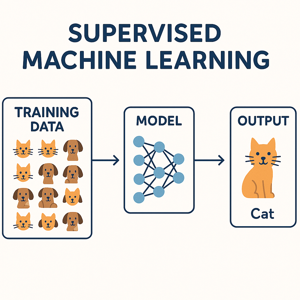
Supervised learning means the machine learns from labelled examples—just like students learning from a teacher who shows them the right answers.

Supervised machine learning is when you teach a computer using examples where you already know the correct answers.

🎓 Think of it like this:

It's like teaching a child with flashcards.

You show a picture of an apple and say, "This is an apple."
You show a picture of a banana and say, "This is a banana."

After seeing many examples, the child learns to recognize apples and bananas on their own.

🧪 In machine learning terms:

The input is the data (like the picture or a sentence).
The output (label) is the correct answer (like "apple" or "banana").
The model learns the relationship between the input and the label.
Later, you can give it new data, and it will try to predict the correct answer.

Here are some real-world examples of supervised machine learning, organized by domain, with brief explanations:

🔐 1. Spam Email Detection

Input (Features): Email content, sender address, subject line.
Output (Label): Spam or Not Spam.
Algorithm Examples: Naive Bayes, Logistic Regression.
Use Case: Gmail, Outlook, and other email services use this to filter junk mail.

🏦 2. Credit Risk Assessment

Input: Age, income, employment status, credit history.
Output: Loan Default Risk (High/Low) or Credit Score.
Algorithm Examples: Decision Trees, Random Forest, XGBoost.
Use Case: Banks use this to approve or reject loan applications.

🛍️ 3. Product Recommendation

Input: User's past purchases, browsing history.
Output: Probability of purchasing a product (Yes/No).
Algorithm Examples: Support Vector Machines (SVM), Logistic Regression.
Use Case: Amazon, Netflix, Flipkart, and other platforms recommend items.

🎓 4. Student Performance Prediction

Input: Attendance, assignment scores, participation.
Output: Final Grade or Pass/Fail.
Algorithm Examples: Linear Regression, K-Nearest Neighbors (KNN).
Use Case: EdTech platforms predict learner outcomes and personalize content.

🏥 5. Disease Diagnosis

Input: Symptoms, blood test results, medical history.
Output: Disease classification (e.g., diabetes, cancer, etc.).
Algorithm Examples: SVM, Neural Networks, Logistic Regression.
Use Case: Medical diagnostic systems and predictive healthcare.

🛣️ 6. Traffic Sign Recognition (Computer Vision)

Input: Image pixels of a road sign.
Output: Sign category (e.g., Stop, Yield, Speed Limit).
Algorithm Examples: Convolutional Neural Networks (CNNs).
Use Case: Used in self-driving cars for decision-making.

🧠 7. Sentiment Analysis

Input: Customer reviews, tweets, or feedback.
Output: Sentiment label (Positive, Negative, Neutral).
Algorithm Examples: Naive Bayes, LSTM (for sequential data).
Use Case: Brands monitor public sentiment using social media analytics tools.

🎯 8. Image Classification

Input: Raw image data.
Output: Image label (e.g., Cat, Dog, Car, etc.).
Algorithm Examples: CNNs, Transfer Learning with ResNet or VGG.
Use Case: Facebook's photo tagging, Instagram content moderation.

📦 9. Inventory Demand Forecasting

Input: Historical sales, seasonality, promotions.
Output: Predicted units needed.
Algorithm Examples: Linear Regression, Time Series Models with supervised extensions.
Use Case: Retail chains optimize stock to reduce overstock or shortages.

🗣️ 10. Speech Emotion Recognition

Input: Audio recordings with extracted features (pitch, tone, etc.).
Output: Emotion label (Happy, Angry, Sad, etc.).
Algorithm Examples: Recurrent Neural Networks (RNN), SVM.
Use Case: Call centers analyze customer tone to improve service.

Here is a detailed overview of the most common supervised learning techniques:

1. Linear Regression

Type: Regression
Use Case: Predicting continuous values (e.g., housing prices).
How it works: Assumes a linear relationship between input variables (X) and the output (y).
Formula:
y=β0+β1x1+β2x2+⋯+βnxn

2. Logistic Regression

Type: Classification
Use Case: Binary or multi-class classification (e.g., spam detection).
How it works: Models the probability that a given input belongs to a particular class using the logistic (sigmoid) function.

3. Decision Trees

Type: Classification/Regression
Use Case: Fraud detection, credit scoring, etc.
How it works: Splits the data into subsets based on feature values using conditions (like yes/no questions), forming a tree structure.

4. Random Forest

Type: Classification/Regression
Use Case: High-accuracy tasks with large datasets.
How it works: Ensemble of multiple decision trees; each tree is trained on a random subset of data and features. Final prediction is made by majority vote or averaging.

5. Support Vector Machines (SVM)

Type: Classification/Regression
Use Case: Image classification, bioinformatics.
How it works: Finds the optimal hyperplane that separates classes with maximum margin. Can handle non-linear data using kernel tricks.

6. K-Nearest Neighbors (K-NN)

Type: Classification/Regression
Use Case: Pattern recognition, recommendation systems.
How it works: Stores all training data; a new input is classified based on the majority class among its k-nearest neighbors.

7. Naïve Bayes

Type: Classification
Use Case: Text classification, spam filtering.
How it works: Applies Bayes' Theorem with strong (naïve) independence assumptions between features.

8. Gradient Boosting Machines (GBM) / XGBoost / LightGBM / CatBoost

Type: Classification/Regression
Use Case: Kaggle competitions, production-level machine learning.
How it works: Sequentially builds models that correct the errors of previous models. Uses decision trees as base learners.

9. Neural Networks (Shallow and Deep)

Type: Classification/Regression
Use Case: Complex problems like image recognition, natural language processing.
How it works: Composed of layers of neurons that transform input data through learned weights and activation functions.

Supervised Machine Learning Technique- Decision Tree

🌳 What is a Decision Tree?

Imagine you're playing a game of 20 Questions, where you ask yes/no questions to guess something. A Decision Tree works in a similar way. It's like a flowchart that helps make a decision step by step by asking questions.

🧠 Simple Example:

What is the weather like?

If it's Sunny, then you ask another question:
- Is it Hot or Cool?
  - If it's Hot → No, don't play outside.
  - If it's Cool → Yes, go play outside!

But if the weather is Rainy, you ask a different question:

How is the wind? Strong or Weak?
- If the wind is Strong → No, it's not safe to play.
- If the wind is Weak → Yes, you can still play.

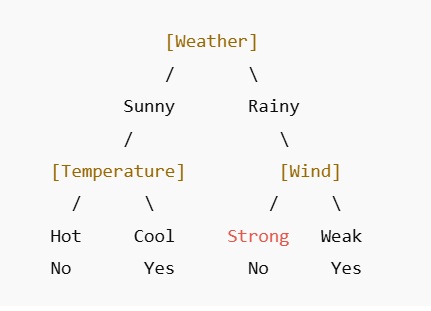
Sample Decision:

Let's say:

It's Sunny
Temperature is Cool

Path:

Weather = Sunny → go left
Temperature = Cool → go right
Result: Yes, play outside

💻 Should You Buy a Laptop?

We'll use 3 simple features:

Budget (High, Low)
Purpose (Gaming, Office)
Brand Trust (Trusted, Unknown)

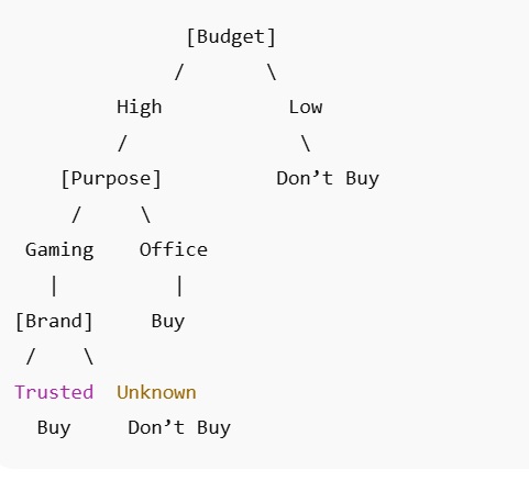
✅ Example Decision:

Let's say:

Budget: High
Purpose: Gaming
Brand: Trusted

Path:

Budget = High → go left
Purpose = Gaming → go left
Brand = Trusted → go left
✅ Result: Buy the laptop

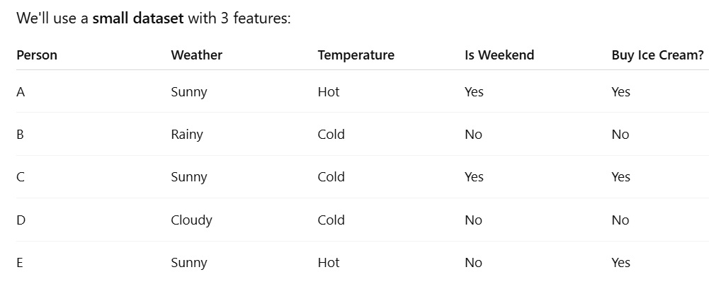
🌳 Goal: Predict if a Person Will Buy Ice Cream

🧠 Creating a decision tree with this data

✅ Step 1: Look at the Target

We want to predict "Buy Ice Cream?" based on other information.

✅ Step 2: Pick the Best Feature to Split

We ask:

Which feature (Weather, Temperature, or Is Weekend) best separates Yes/No?

Let's try Weather first:

When Weather = Sunny → A, C, E → All "Yes"
When Weather = Rainy or Cloudy → B, D → Both "No"

💡 Perfect split! Weather clearly separates the Yes and No groups.

So we make Weather our first question.

Step 3: Draw the Decision Tree

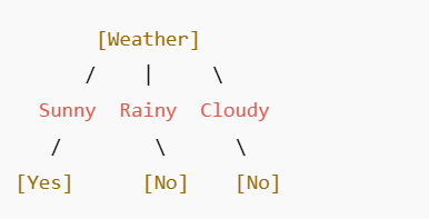
Done! Our tree says:

If Weather = Sunny → Yes
If Weather = Rainy or Cloudy → No

✅ Test It:

New person:

Weather = Sunny
Temperature = Cold
Is Weekend = No

Prediction: → The tree says "Sunny" → So, Yes, they'll buy ice cream!

Gini Impurity Formula

Gini impurity is a metric used in decision trees to measure how often a randomly chosen element from a set would be incorrectly labeled if it were randomly labeled according to the distribution of labels in the subset.

The general formula for Gini impurity is:

Gini(S) = 1 − Σ pᵢ²

where:

S is a dataset or node in a decision tree,
pᵢ is the proportion of samples in S that belong to class i,
the summation Σ is taken over all classes.

For a binary classification problem with class probabilities p and 1 − p, the Gini impurity simplifies to:

Gini(S) = 1 − (p² + (1 − p)²) = 2p(1 − p)

Lower Gini impurity values indicate purer nodes, which are preferred when building decision trees for classification.

Lets calculate the gini impurity for above example (Goal: Predict if a Person Will Buy Ice Cream)

Step 1: Full Dataset Gini

Classes: Buy Ice Cream? = Yes / No

Counts: Yes = 3, No = 2

First, compute the class probabilities:

p(Yes) = 3 / 5 = 0.6
p(No) = 2 / 5 = 0.4

The formula for Gini impurity is:

Gini = 1 − Σ p(i)²

Apply the probabilities:

p(Yes)² = 0.6² = 0.36
p(No)² = 0.4² = 0.16
Σ p(i)² = 0.36 + 0.16 = 0.52

Gini impurity = 1 − 0.52 = 0.48

Step 2: Gini for each Weather split

Weather = Sunny

Rows: A, C, E → 3 samples

Buy Ice Cream:

Yes = 3
No = 0

The Gini impurity formula for a node is:

Gini = 1 − Σ(pᵢ²), where pᵢ is the proportion of each class in the node.

In this case:

p(Yes) = 3 / 3 = 1
p(No) = 0 / 3 = 0

Now compute Gini impurity:

Gini = 1 − (1² + 0²) = 1 − (1 + 0) = 1 − 1 = 0

A Gini impurity of 0 means the node is perfectly pure, containing only "Yes" outcomes for buying ice cream.

Gini Impurity for Weather = Rainy

For the subset where Weather = Rainy, there is a total of 1 sample.

Class distribution for the target Buy Ice Cream is:

Yes = 0
No = 1

The Gini impurity formula is:

Gini = 1 − Σ(pᵢ²)

Here, the probabilities are:

p(Yes) = 0 / 1 = 0
p(No) = 1 / 1 = 1

So the Gini impurity is:

Gini = 1 − (0² + 1²) = 1 − (0 + 1) = 0

The node for Weather = Rainy is therefore perfectly pure with a Gini impurity of 0.

Weather = Cloudy

Rows: D → 1 sample

Buy Ice Cream:

Yes = 0
No = 1

Gini = 1 − (0² + 1²) = 1 − (0 + 1) = 0✔ Pure

Step 3: Weighted Gini After Splitting on Weather

Group sizes:

Sunny = 3
Rainy = 1
Cloudy = 1

Ginisplit=3/5(0)+1/5(0)+1/5(0) =0

Step 4: Gini Gain (Reduction)

Gain=Gini original−Gini split =0.48−0=0.48

⭐ Conclusion

Weather gives a perfect split because all groups become pure:

Weather Buy Ice Cream?
Sunny Always Yes
Rainy Always No
Cloudy Always No

🌲Supervised Machine Learning Technique - Random Forest

A Random Forest is like a team of decision trees that work together to make better decisions. Imagine asking not just one friend for advice, but a group of friends and then taking a vote. That's how a Random Forest works!

🤔 Why use Random Forest instead of just one tree?

Decision trees can sometimes make mistakes or overfit (learn too much from training data).
A random forest builds many trees and combines their results to reduce error and increase accuracy.

🔍 How It Works (Layman Terms):

You create lots of decision trees.
Each tree sees a random part of the data (this is called bootstrapping).
Each tree also looks at only a random set of features when making splits.
Each tree gives a prediction.
The forest takes a vote:
- For classification: it picks the class with majority vote.
- For regression: it takes the average prediction.

📦 Real-Life Example:

Should a bank approve a loan?

Instead of relying on one decision tree, the bank builds 100 decision trees, each looking at slightly different customer data (like income, job history, credit score, etc.).
Each tree makes a yes/no decision.
The majority vote (e.g., 75 say YES, 25 say NO) is the final decision: Approve the loan.

✅ Benefits:

Very accurate and robust.
Works well with both classification and regression tasks.
Handles missing data and noisy datasets.

⚠️ Downsides:

Slower than a single tree (more trees = more time).
Less interpretable (you can't easily draw the whole forest).

Here's a simple example of Random Forest in action—explained in an easy-to-understand way

💡 Scenario: Predict if a person will buy a mobile phone

We have a small dataset with these features:

Age
Income
Likes Tech
Will Buy Phone? (Target: Yes/No)

Sample Data

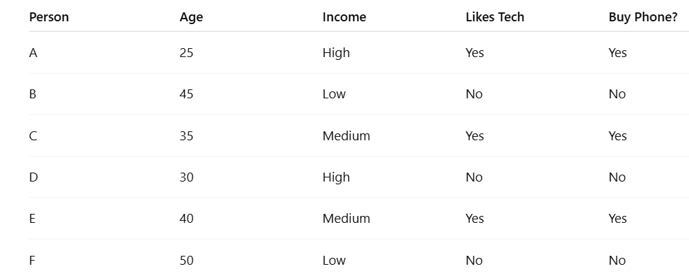
🌲 How Random Forest Works:

Let's say we build 3 decision trees in the forest.

📌 Tree 1 might learn:

If Age < 40 AND Likes Tech → Yes
Else → No

📌 Tree 2 might learn:

If Income is High AND Likes Tech→ Yes
Else → No

📌 Tree 3 might learn:

If Likes Tech = Yes → Yes
Else → No

🔍 Each Tree Predicts:

Tree 1: Age < 40 & Likes Tech → Yes
Tree 2: Income is not High → No
Tree 3: Likes Tech = Yes → Yes

🗳️ Final Vote:

Yes → 2 trees
No → 1 tree

✅ Random Forest Prediction: Yes (buy phone)

Regression Tree Example

Scenario : A company wants to predict the sales (in thousands) of a product based on advertising spend (in $1000s).

Advertising spend values of 1, 2, 3, 4, and 5 correspond to sales values of 3, 4, 6, 8, and 10 respectively.

Step 1: Start at the root node

All data points are at the root.
Calculate the average sales at root:

Mean(Y)=(3+4+6+8+10)/5=31/5=6.2

This is our prediction if we don't split.

Step 2: Choose a split

Regression trees choose splits to minimize variance in each child node.
Let's try splitting at X ≤ 3 and X > 3.

Left Node (X ≤ 3):
Y values = 3, 4, 6
Mean = (3+4+6)/3 = 13/3 ≈ 4.33
Variance = [(3−4.33)2+(4−4.33)2+(6−4.33)2]/3≈2.33

Right Node (X > 3):
Y values = 8, 10
Mean = (8+10)/2 = 9
Variance = [(8−9)2+(10−9)2]/2=1

Total variance after split: 2.33 + 1 = 3.33
This is lower than root variance, so we split here.

Step 3: Build the tree

Root: Predict 6.2 (if no split)
Split at X = 3:

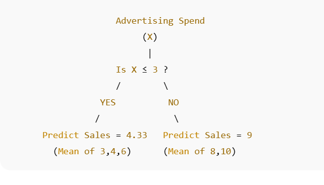
Step 4: Make predictions

If advertising = 2 → X ≤ 3 → predict 4.33
If advertising = 5 → X > 3 → predict 9

A regression tree predicts continuous values by splitting data to minimize variance, and each leaf node outputs the mean of the target variable.

MCQs on Decision Trees

1. What type of machine learning task are decision trees primarily used for?
A) Clustering
B) Classification and Regression
C) Dimensionality reduction
D) Reinforcement learning

Answer: B
Explanation: Decision trees can handle both classification (categorical output) and regression (continuous output).

2. In a decision tree, what does each internal node represent?
A) A class label
B) A test on an attribute
C) The final prediction
D) Random noise

Answer: B
Explanation: Internal nodes test attributes/features to split the data.

3. What does a leaf node represent in a decision tree?
A) A test on a feature
B) A subset of data
C) A class label or a regression value
D) A random split

Answer: C
Explanation: Leaf nodes provide the predicted outcome for a data instance.

7. Overfitting in decision trees occurs when:
A) The tree is too shallow
B) The tree has too many branches capturing noise
C) The data has no labels
D) The features are categorical

Answer: B
Explanation: A very deep tree can model noise in the training data, leading to overfitting.

8. Which method helps to reduce overfitting in decision trees?
A) Pruning
B) Feature scaling
C) Increasing tree depth
D) Random initialization

Answer: A
Explanation: Pruning removes nodes that do not provide significant information gain.

9. Which of the following is a disadvantage of decision trees?
A) Easy to interpret
B) Handles both numerical and categorical data
C) Prone to overfitting
D) Requires little data preparation

Answer: C
Explanation: While decision trees are intuitive, they can overfit if not pruned properly.

10. Which of the following is true about Gini Index?
A) Lower Gini Index indicates higher impurity
B) Higher Gini Index indicates lower impurity
C) Lower Gini Index indicates higher purity
D) Gini Index is not used in decision trees

Answer: C
Explanation: Gini Index measures impurity; lower values indicate more homogeneous groups.

12. Decision trees can handle:
A) Only numerical features
B) Only categorical features
C) Both numerical and categorical features
D) None of the above

Answer: C
Explanation: Decision trees can split both types of attributes effectively.

14. Which ensemble technique uses multiple decision trees?
A) SVM
B) Random Forest
C) Naive Bayes
D) KNN

Answer: B
Explanation: Random Forest combines multiple trees to reduce overfitting and improve accuracy.

15. How does Random Forest improve over a single decision tree?
A) By pruning
B) By bagging and averaging multiple trees
C) By using gradient descent
D) By normalizing data

Answer: B
Explanation: Bagging (bootstrap aggregation) reduces variance and increases predictive performance.

16. In regression trees, which criterion is used for splitting?
A) Information Gain
B) Gini Index
C) Variance Reduction
D) Euclidean distance

Answer: C
Explanation: Regression trees aim to minimize variance within nodes.

17. Which of the following can be used to visualize decision trees?
A) Heatmap
B) Dendrogram
C) Tree diagram
D) Scatter plot

Answer: C
Explanation: A tree diagram shows nodes, splits, and leaves clearly.

18. A high depth of a decision tree usually results in:
A) Underfitting
B) Overfitting
C) High bias
D) Low variance

Answer: B
Explanation: Deep trees tend to overfit by memorizing training data.

19. Which Python library is commonly used for decision tree implementation?
A) NumPy
B) Scikit-learn
C) TensorFlow
D) Matplotlib

Answer: B
Explanation: Scikit-learn provides DecisionTreeClassifier and DecisionTreeRegressor.

20. What is pruning in decision trees?
A) Adding more nodes to the tree
B) Removing irrelevant or less significant branches
C) Splitting nodes using Gini Index
D) Normalizing features

Answer: B
Explanation: Pruning reduces complexity and improves generalization.

22. Decision trees are:
A) Parametric models
B) Non-parametric models
C) Both A and B
D) None

Answer: B
Explanation: Decision trees make no assumptions about the data distribution.

23. What is the main disadvantage of using decision trees on very large datasets?
A) They cannot handle categorical features
B) They are computationally expensive and prone to overfitting
C) They cannot handle missing data
D) They are slow to interpret

Answer: B
Explanation: Large trees can become very complex, increasing computational cost and overfitting risk.

26. Which of the following is an advantage of decision trees?
A) Hard to interpret
B) Works only on linear relationships
C) Can capture nonlinear relationships and interactions
D) Cannot handle categorical data

Answer: C
Explanation: Decision trees are flexible and can model complex patterns.

28. Ensemble of decision trees reduces:
A) Bias
B) Variance
C) Both bias and variance
D) Neither

Answer: B

Explanation: Techniques like bagging reduce variance while maintaining low bias.

29. A decision tree with only one node (the root) is an example of:
A) Underfitting
B) Overfitting
C) Perfect fit
D) Random forest

Answer: A
Explanation: Such a tree is too simple to capture data patterns, causing underfitting.

30. Which of the following is a stopping criterion when building a decision tree?
A) Maximum depth reached
B) Minimum samples per leaf
C) Node purity threshold
D) All of the above

Answer: D
Explanation: All these conditions can stop further splitting.

33. Bagging stands for:
A) Bootstrap Aggregation
B) Binary Aggregation
C) Basic Averaging
D) Boosted Accuracy

Answer: A
Explanation: Bagging uses bootstrapped samples to train multiple models and aggregate results.

34. Which ensemble method builds trees sequentially to correct errors of previous trees?
A) Random Forest
B) Boosting
C) Bagging
D) PCA

Answer: B
Explanation: Boosting improves performance by focusing on misclassified samples sequentially.

35. Which of the following is true about splitting attributes?
A) Decision tree always splits at median
B) Splits are chosen to maximize class purity
C) Attributes are selected randomly
D) Only categorical attributes are used

Answer: B
Explanation: Splits are chosen to create the most homogeneous child nodes.

38. Decision tree complexity can be controlled using:
A) Max depth
B) Min samples per leaf
C) Pruning
D) All of the above

Answer: D
Explanation: All are common hyperparameters to prevent overfitting.

39. Random Forest reduces overfitting by:
A) Using a single deep tree
B) Random feature selection and averaging multiple trees
C) Pruning one tree
D) Reducing data size

Answer: B
Explanation: Random feature selection and bagging reduce correlation and variance among trees.

40. Which of the following statements is true?
A) Decision trees cannot model nonlinear relationships
B) Decision trees always generalize well to unseen data
C) Decision trees are easy to interpret but prone to overfitting
D) Decision trees require data normalization

Answer: C
Explanation: Trees are interpretable but need careful tuning to avoid overfitting.